 Finding the Equation Using a TI83+ Method 2: Using the TI83+ or TI84 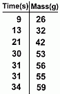
 At the left is the data that we want to enter in the calculator.
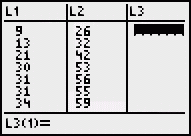
The numbers get entered into two lists: L1 and L2. To do this, press the STAT key, and then choose the first menu item, EDIT by pressing ENTER. After the numbers have been entered into each list, you'll see a screen on your calculator like the one at the right. 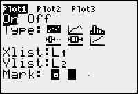
 Next, you need to turn on 'StatPlot' to graph the points.
Press 2nd and Y= (this accesses STATPLOT).
Next, you need to turn on 'StatPlot' to graph the points.
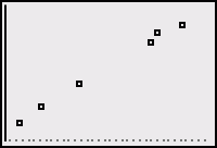
Press 2nd and Y= (this accesses STATPLOT).Press ENTER for choice 1. On this screen (see the picture at left), make sure Plot1 and On are both black, as well as the first graph type. Press the ZOOM key and choose #9: ZoomStat, and press ENTER. You'll see the scatterplot, shown at the right. Now we want to make the calculator show the line of best fit, and find its equation. We'll access the Linear Regression function in the calculator: 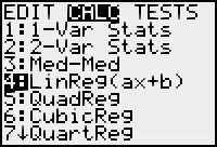 First, press the STAT key. Use the right arrow to get the second menu type at the top, CALC. You'll see a menu like the picture at the left.
 Use the down arrow and ENTER to pick #4: LinReg(ax+b). You'll see the words The calculator is now waiting for you to tell it which lists to pick the data from, and how to graph it. You're going to tell it L1, L2, and Y1: After LinReg(ax+b) on the screen press L1 (2nd - 1), then a comma (the comma key is just above the 7 key), then L2 (2nd - 2), then a comma again, and finally Y1. You get Y1 from the variables menu: press VARS, then go right to get the Y-VARS menu, press ENTER for choice #1 (Function), and ENTER again for choice #1 (Y1). 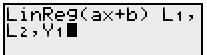 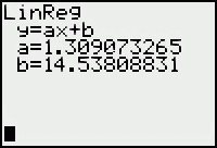
 You will now see the screen on the left. This is the equation of the line of best fit; filling in the values
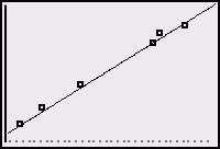
 y = 1.309073265x + 14.53808831 To see the line on the graph, just press the GRAPH key. What you'll see is shown at the right. You can judge how well the line fits the points by how close they lie to the line; in this example there is a very strong correlation ... it's almost perfect. But everything would work just the same even if the points were more scattered. If you'd like to use your calculator to identify or predict points, press the TRACE key and then the UP arrow; then if you use the left/right arrows you can move a cursor along the line to identify whatever point you want; its coordinates are shown at the bottom of the screen. You may have noticed that this equation is slightly different than the one we found on the previous page without the use of a calculator. That's because on the previous page we located the line by 'eye' and were probably off a little. Here, the calculator's choice for the line's location and the calculator's version of the equation can both be considered more accurate. When you're all done, you'll want to restore the calculator's default settings. Here's how: - Press the Y= key, and then CLEAR, to remove the stored equation. - Press the STAT key, scroll down to ClrList, and press ENTER. Tell it to clear both lists by typing L1, L2 and pressing ENTER. - Turn off STATPLOT: press 2nd and y=, then press ENTER, then use the right arrow to choose OFF and press ENTER again. Then press QUIT (2nd - mode) - Reset the graph window: press WINDOW and enter the values -10, 10, 1, -10, 10, 1,1 If you don't have anything stored in your calculator, there's a quicker way to do all of the above ... you can just reset the calculator. Press MEM (2nd - +). Scroll down to #7: Reset and press ENTER. Press ENTER again to choose ALL RAM. Scroll down to #2: Reset and press ENTER once more. Then press ENTER a final time to clear the screen. Although this procedure may seem tedious, it's a handy one to know, since every once in a while your calculator may develop a glitch where things don't work properly, or you keep getting error messages. Resetting the calculator usually fixes these problems. After a RESET, you might want to go to MODE and put the angle setting (the third menu item) back on DEGREE, so it will be ready for any trigonometry problems you might need to do in the future. |